


This article explores the use of the functions .UnivariateSpline() and .LSQUnivariateSpline(), from the Scipy package.
What Are Splines?
Splines are mathematical functions that describe an ensemble of polynomials which are interconnected with each other in specific points called the knots of the spline.
They’re used to interpolate a set of data points with a function that shows a continuity among the considered range; this also means that the splines will generate a smooth function, which avoid abrupt changes in slope.
Compared to the more classical fitting methods, the main advantage of splines is that the polynomial equation is not the same throughout the whole range of data points.
Instead, the fitting function can change from one interval to the subsequent one, allowing for fitting and interpolation of very complicated point distributions. In this article we will see:
- i) how to generate a spline function to fit a given set of data points,
- ii) which functions we can then use to extrapolate the value of points within the fitted range,
- iii) how to improve the fitting, and
- iv) how to calculate the related error.
Splines — A Mathematical Perspective
In mathematics, splines are functions described by an ensemble of polynomials.
Even if splines seem to be described by a single equation, they are defined by different polynomial functions which holds over a specific range of points, whose extremes are called knots. Each knot hence represents a change in the polynomial function that is describing the shape of the spline in that specific interval.
One of the main characteristics of splines is their continuity; they are continuous along the entire interval in which they are defined; this allows for the generation of a smooth curve, that fit our set of data points.
One of the main advantages of using splines for fitting problems, instead of single polynomials, is the possibility of using lower degree polynomial functions to describe very complicated functions.
Indeed, if we wanted to use a single polynomial function, the degree of the polynomial usually increases with the complexity of the function that has to be described; increasing the degree of the fitting polynomial could introduce unwanted errors in the problem.
Here is a nice video that explain in simple terms this issue:
Splines avoid this by varying the fitting equation over the different intervals that characterize the initial set of data points. From an historical point of view, the word “Spline” comes from the flexible spline devices that were exploited by the shipbuilders to draw smooth shapes in the designing of vessels. Nowadays they also find large application as fundamental tools in lots of CAD software (https://en.wikipedia.org/wiki/Spline_(mathematics) ).
Scipy.UnivariateSpline
In the first part of this article we explore the function .UnivariateSpline(); which can be used to fit a spline of a specific degree to some data points.
To understand how this function works, we start by generating our initial x and y arrays of data points. The x array (called “x”), is defined by using the np.linspace() function; the y array is defined by exploiting the np.random function called .randn(), which return a sample from the standard normal distribution.
See: https://numpy.org/devdocs/reference/random/generated/numpy.random.randn.html for additional documentation.
import matplotlib.pyplot as plt

from scipy.interpolate import UnivariateSpline, LSQUnivariateSpline

import numpy as np #x and y array definition (initial set of data points)

x = np.linspace(0, 10, 30)

y = np.sin(0.5*x)*np.sin(x*np.random.randn(30))
Once we have defined the initial set of data points, we can call the function .UnivariateSpline(), from the Scipy package and calculate the spline that best fits our points.
While the procedure is rather simple, understanding the fundamental parameters that define the spline function that we want to create, might generate some confusion; to this purpose, it is better to analyze in detail the main input parameters that can be defined when calling the function in our code.
As can be also seen in the documentation (https://docs.scipy.org/doc/scipy/reference/generated/scipy.interpolate.UnivariateSpline.html), the .UnivariateSpline() function accepts as mandatory inputs the x and y arrays of data points that we want to fit.
In most cases, our aim is to fit complicated functions and to this purpose, other parameters must be specified.
One of the most important parameters is “k”, which refers to the degree of the polynomials that define the spline segments. “k” can vary between one and five; increasing the degree of the polynomials allows a better fitting of more complicated functions; however, in order not to introduce artifacts in our fit; the best practice is to use the lower degree that allows for the better fitting procedure.
Another relevant parameter is “s”, it’s a float number which defines the so-called smoothing factor, which directly affects the number of knots present in the spline. More precisely, once we fix a specific value of “s”, the number of knots will be increased until the difference between the value of the original data points in the y array and their respective datapoints along the spline is less than the value of “s” (see documentation for the mathematical formula). It can be understood that the lower the value of “s”, the higher the fitting accuracy and (most of the times) the n° of knots, since we are asking for a smaller difference between the original points and the fitted ones.
Now that the parameters that governs the shape of our spline are clearer, we can return to the code and define the spline function. In particular, we will give as input arrays the “x” and “y” arrays previously defined; the value of the smoothing factor is initially set to five while the parameter “k” is left with the default value, which is three.
#spline definition spline = UnivariateSpline(x, y, s = 5)
The output of the .UnivariateSpline() function is the function that fit the given set of data points. At this point, we can generate a denser x array, called “x_spline” and evaluate the respective values on the y axis using the spline function just defined; we then store them in the array “y_spline” and generate the plot.
x_spline = np.linspace(0, 10, 1000)

y_spline = spline(x_spline)

#Plotting

fig = plt.figure()

ax = fig.subplots()

ax.scatter(x, y)

ax.plot(x_spline, y_spline, 'g')

plt.show()
The result of this procedure is displayed in Figure 1.
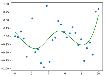
As can be seen from Figure 1, the obtained spline gives a really bad fit of our initial data points; the main reason is the relatively high value that was assigned to the smoothing factor; we will now explore a possible strategy for improving our spline, without introducing exaggerated alterations.
One of the best way to improve this situation is to exploit the method .set_smoothing_factor(s); which continues the spline calculation according to a new smoothing factor (“s”, given as the only input), without altering the knots already found during the last call. This represents a convenient strategy, indeed, splines might be very sensitive to changes in the smoothing factor; this means that changing the smoothing function, directly in the .UnivariateSpline() calling, might alter significantly the output result in term of the spline shape (keep in mind that our goal is always to obtain the best fit with the simplest spline possible). The following code lines describe the definition of a new and more accurate spline function, with a smoothing factor equal to 0.5.
After the application of the above-mentioned method, the procedure is identical to the one described for generating the first spline.
# Changing the smoothing factor for a better fit

spline.set_smoothing_factor(0.05)

y_spline2 = spline(x_spline)
We conclude by plotting the result; Figure 2 display the final output, the new spline is the blue curve, plotted together with the old one (green curve) and the initial data points (light blue points).
#Plotting

fig = plt.figure()

ax = fig.subplots()

ax.scatter(x, y)

ax.plot(x_spline, y_spline, 'g', alpha =0.5)

ax.plot(x_spline, y_spline2, 'b')

plt.show()
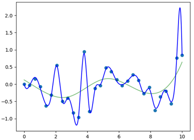
As can be seen from Figure 2, the newly generated spline function well describes the initial data points and still pass by the knots that were found in the initial call (data points common to both the two spline functions)
We conclude this part by illustrating some useful methods that can be used after the generation of the correct spline function, for describing our data points. The first of these methods is called “.__call__(x)”, which allows evaluating the value of specific points on the spline, given in the form of a list or single number. The following lines describe the application of this methods (we evaluate the the spline for a value of 2 in the x-axis).
#evaluate point along the spline

print(spline.__call__(2))
The result of the print command is 0.5029480519149454. Another important method is .get_residual(), which allows obtaining the weighted sum of squared residuals of the spline approximation (more simply, an evaluation of the error in the fitting procedure).
#get the residuals

print(spline.get_residual())
The result for this case is 0.049997585478530546. In some applications, it could be of some interest to calculate the definite integral of the spline (i.e. the area underneath the spline curve between a specific range along the x-axis); to do this, the method .integral(a,b) represents the simplest solution; “a” and “b” are the lower and upper limits along the x-axis between which we want to evaluate the area (in this case we calculate the area underneath the spline, between 1 and 2). Application of this method is illustrated in the following lines.
#definite integral of the spline

print(spline.integral(1,2))
The result of the integration is -0.2935394976155577. The last method allows obtaining the values of the points in which the spline crosses the x-axis, i.e. the solutions to the equations defining the spline function. The method is called .roots(), its application is shown in the following lines.
#finding the roots of the spline function

print(spline.roots())
The output of this last line is an array containing the values of the points for which the spline crosses the x-axis, namely:
[1.21877130e-03 3.90089909e-01 9.40446113e-01 1.82311679e+00 2.26648393e+00 3.59588983e+00 3.99603385e+00 4.84430942e+00 6.04000192e+00 6.29857365e+00 7.33532448e+00 9.54966590e+00]
Scipy.LSQUnivariateSpline
In the last part of this article, we introduce .LSQUnivariateSpline(), another function that can be used for spline generation. From a practical point of view, it works similarly to .UnivariateSpline(), indeed as we will see, there are very few differences in how we call and define it in our script.
The fundamental difference between this function and the previous one, is that .LSQUnivariateSpline() allows generating spline curves by directly controlling the number and the position of the knots.
This means that we have the full control of the knots that will define the spline; differently, in the previous case, the number of knots was indirectly regulated through the choice of the smoothing factor. In order to appreciate how our spline will change by increasing the number of knots, we start by defining two different arrays, “t” and “t1”, t1 is the denser array.
#LSQUnivariateSpline

t = np.array([0.5, 1, 2.5])

t1 = np.linspace(1, 9, 20)
The function .LSQUnivariateSpline() accepts as mandatory input, the x, y arrays and the array “t”, which contains the coordinates of the knots that will define our spline. An important condition that has to be kept in mind is that the coordinates of the knots must be located within the range of the x array.
In our case, we will use the same x and y arrays employed for the previous case. At this point we have to call the function twice, in order to show the difference between the two set of knots arrays. In addition, we specify the parameter “k”, which again refers to the degree of the polynomials that describe the spline.
LSQUspline = LSQUnivariateSpline(x, y, t1, k = 4)

LSQUspline1 = LSQUnivariateSpline(x, y, t, k = 4)
Our final task is to plot the two splines, together with the original data points. We will generate the arrays containing the y values of the two splines directly in the plotting command.
#Plotting

plt.scatter(x, y, s=8)

plt.plot(x_spline, LSQUspline(x_spline), color = 'b')

plt.plot(x_spline, LSQUspline1(x_spline), color = 'g')

plt.show()
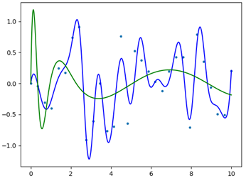
The final result is displayed in Figure 3; as can be seen, by increasing the number of knots, the spline function better approximates our data points. If we check carefully, both the splines pass for the knots specified in the “t” and “t1” arrays, respectively. Most of the methods previously shown for .UnivariateSpline() work on this function too (for additional documentation please refer to https://docs.scipy.org/doc/scipy/reference/generated/scipy.interpolate.LSQUnivariateSpline.html ).
Conclusion
To conclude, in this article, we explored spline functions, their power and versatility.
One thing that is important to keep in mind is that when we are using splines for fitting and interpolating a given set of data points, we should never exceeds with the degree of the polynomials that define the spline; this is to avoid unwanted errors and incorrect interpretation of the initial data.
The process has to be accurately refined, possibly through repetitive iterations to double check the validity of the generated output.
The post Fitting Data With Scipy’s UnivariateSpline() and LSQUnivariateSpline() first appeared on Finxter.
https://www.sickgaming.net/blog/2020/12/...atespline/